

Python for Data Analysis: Machine Learning with Scikit-Learn
Written by Yasin TANIŞ

Introduction
Machine learning is the branch of science that lets computers learn from data and make predictions, and it is used across many industries today. In this article we look at Scikit-Learn, one of the most widely used Python libraries for building machine learning applications.
What Scikit-Learn is
Scikit-Learn is a machine learning library that offers simple, efficient tools for Python. It includes both supervised and unsupervised learning algorithms.
Installation
Before we start, the library needs to be installed. If it is not on your system yet, install it with this command:
pip install scikit-learnNote: the examples here are deliberately simple to illustrate the concepts; they are not always the best metric or method for every scenario.
Supervised learning
Supervised learning works with labelled data: the outcomes (labels) of the examples are known, so the model can learn to predict them.
Logistic regression
Logistic regression is a widely used algorithm for classification problems.
from sklearn.datasets import load_iris
from sklearn.model_selection import train_test_split
from sklearn.linear_model import LogisticRegression
from sklearn.metrics import accuracy_score
# Veri setini yükle
iris = load_iris()
X = iris.data
y = iris.target
# Veriyi eğitim ve test olarak ayır
X_train, X_test, y_train, y_test = train_test_split(X, y, test_size=0.2, random_state=42)
# Model oluştur ve eğit
model = LogisticRegression(max_iter=200)
model.fit(X_train, y_train)
# Tahmin yap ve doğruluğu ölç
y_pred = model.predict(X_test)
accuracy = accuracy_score(y_test, y_pred)
print(f'Model accuracy: {accuracy}')
Model Accuracy : 1.0This code loads the Iris data set, splits it into features and target, trains the model and prints its accuracy.
Decision trees
Decision trees are a powerful algorithm for both classification and regression.
from sklearn.tree import DecisionTreeClassifier

# Model oluştur ve eğit
tree_model = DecisionTreeClassifier(random_state=42)
tree_model.fit(X_train, y_train)

# Tahmin yap ve doğruluğu ölç
y_pred_tree = tree_model.predict(X_test)
accuracy_tree = accuracy_score(y_test, y_pred_tree)

print(f'Decision Tree Model accuracy: {accuracy_tree}')
Decision Tree Model Accuracy: 1.0Unsupervised learning
Unsupervised learning does not use labelled data; the model tries to learn the structure of the data itself.
K-Means clustering
K-Means is a common clustering algorithm that splits data into k clusters.
from sklearn.cluster import KMeans
import matplotlib.pyplot as plt

# Örnek veri seti oluştur
from sklearn.datasets import make_blobs
X, _ = make_blobs(n_samples=300, centers=4, random_state=42)

# Model oluştur ve eğit
kmeans = KMeans(n_clusters=4, random_state=42)
kmeans.fit(X)

# Tahmin yap ve kümeleri görselleştir
y_kmeans = kmeans.predict(X)

plt.scatter(X[:, 0], X[:, 1], c=y_kmeans, s=50, cmap='viridis')
centers = kmeans.cluster_centers_
plt.scatter(centers[:, 0], centers[:, 1], c='red', s=200, alpha=0.75)
plt.title('K-Means Clustering')
plt.show()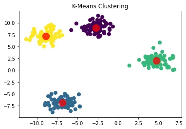
Principal component analysis (PCA)
PCA is a technique for reducing high-dimensional data to fewer dimensions.
from sklearn.decomposition import PCA

# Model oluştur ve eğit
pca = PCA(n_components=2)
X_pca = pca.fit_transform(X)

plt.scatter(X_pca[:, 0], X_pca[:, 1], c=y_kmeans, s=50, cmap='viridis')
plt.title('PCA Visualization')
plt.show()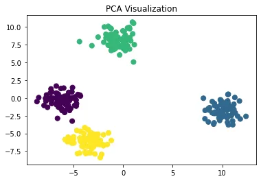
Hyperparameter tuning
Hyperparameter tuning is an important step in getting the best performance from a model. Scikit-Learn's GridSearchCV class makes it easy.
from sklearn.model_selection import GridSearchCV
from sklearn.svm import SVC

# Parametre uzayını tanımla
param_grid = {'C': [0.1, 1, 10], 'kernel': ['rbf', 'linear']}

# Grid search nesnesi oluştur
grid_search = GridSearchCV(SVC(), param_grid, cv=5)

# Grid search'ü uygula
grid_search.fit(X_train, y_train)

print("En iyi parametreler:", grid_search.best_params_)
print("En iyi skor:", grid_search.best_score_)
En iyi parametreler: {'C': 1, 'kernel': 'linear'}
En iyi skor: 0.9583333333333334(The output labels are in Turkish because the original code prints them that way: "best parameters" and "best score".)
Cross-validation
Cross-validation is an important technique for measuring how well a model generalizes to new data.
import numpy as np

# Örnek sayısını en küçük olan veri setine eşitleyin
min_samples = min(X.shape[0], y.shape[0])

# Rastgele örnekleme yapın
np.random.seed(42)  # Tekrarlanabilirlik için
indices = np.random.choice(X.shape[0], min_samples, replace=False)
X = X[indices]
y = y[:min_samples]  # y zaten daha küçük

print("New X shape:", X.shape)
print("New y shape:", y.shape)
New X shape: (150, 2)
New y shape: (150,)from sklearn.model_selection import cross_val_score
from sklearn.linear_model import LogisticRegression
# Lojistik regresyon modelini oluştur
log_reg = LogisticRegression()
# 5-fold cross-validation uygula
scores = cross_val_score(log_reg, X, y, cv=5)
print("Cross-validation skorları:", scores)
print("Ortalama skor:", scores.mean())Cross-validation skorları: [0.33333333 0.4 0.26666667 0.36666667 0.3 ]
Ortalama skor: 0.33333333333333337Correction note: the low scores here come from the previous step, not from the model. The resampling code shuffles the rows of X but does not shuffle the labels in y the same way, so the labels no longer match the rows and the model drops to chance level (about 0.33 with three classes). Skip that step, or select X and y with the same indices, and the scores go back up. The metrics and pipeline results below are low for the same reason, since they use the same data.
Feature selection and engineering
Feature selection and engineering play a critical role in model performance. Scikit-Learn provides tools that make these steps easier.
from sklearn.feature_selection import SelectKBest, f_classif

# En iyi 2 özelliği seç
selector = SelectKBest(f_classif, k=2)
X_new = selector.fit_transform(X, y)

print("Seçilen özellikler:", selector.get_support())
Seçilen özellikler: [ True True]Model interpretability
For models such as decision trees in particular, it matters to understand how the model reaches its decisions.
from sklearn.tree import plot_tree
import matplotlib.pyplot as plt

# Karar ağacını görselleştir
plt.figure(figsize=(20,10))
plot_tree(tree_model, feature_names=iris.feature_names, class_names=iris.target_names, filled=True)
plt.show()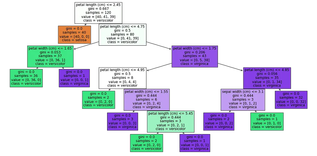
The chart shows the decision tree of a classifier trained on the Iris data set. The tree separates the setosa, versicolor and virginica classes using a few rules:
- Root node: condition petal length ≤ 2.45 cm; Gini 0.667; 120 samples, split [40, 41, 39]. The classes are most mixed here.
- Left child: Gini 0.0; all 40 samples are setosa. A single rule separates setosa completely.
- Right child (petal length > 2.45 cm): Gini 0.5; 80 samples, split [0, 41, 39]. Versicolor and virginica are still mixed.
- Finer split: condition petal length ≤ 4.75 cm; Gini 0.206; 43 samples, split [0, 5, 38], mostly virginica.
- Lower nodes: condition petal width ≤ 1.75 cm; Gini 0.0; all 35 samples are virginica.
Each node shows the Gini coefficient, the number of samples and the class split, so you can follow exactly which feature the model uses at which point and how it decides.
Ensemble methods
Ensemble methods combine several models to make stronger predictions. Random Forest is one of the most popular.
from sklearn.ensemble import RandomForestClassifier

# Random Forest modeli oluştur ve eğit
rf_model = RandomForestClassifier(n_estimators=100, random_state=42)
rf_model.fit(X_train, y_train)

# Tahmin yap ve doğruluğu ölç
y_pred_rf = rf_model.predict(X_test)
accuracy_rf = accuracy_score(y_test, y_pred_rf)

print(f'Random Forest Model accuracy: {accuracy_rf}')
Random Forest Model accuracy: 1.0Evaluation metrics
Beyond accuracy, other evaluation metrics matter too.
from sklearn.model_selection import train_test_split
from sklearn.linear_model import LogisticRegression
from sklearn.metrics import classification_report, confusion_matrix

# Veri setini ayır
X_train, X_test, y_train, y_test = train_test_split(X, y, test_size=0.3, random_state=42)

# Modeli eğit
log_reg = LogisticRegression()
log_reg.fit(X_train, y_train)

# Tahminler yap
y_pred_log = log_reg.predict(X_test)

# Sınıflandırma raporu oluştur
print(classification_report(y_test, y_pred_log, target_names=iris.target_names))

# Confusion matrix oluştur
cm = confusion_matrix(y_test, y_pred_log)
print("Confusion Matrix:\n", cm)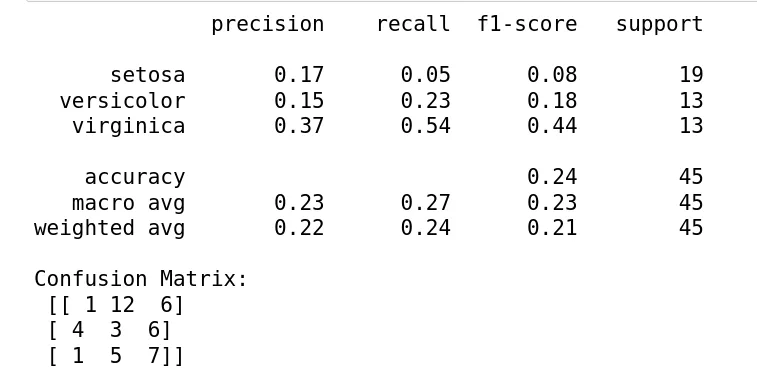
These results show the performance of a model trained on the shuffled data from above:
- Precision, the share of positive predictions that are correct: setosa 17%, versicolor 15%, virginica 37%.
- Recall, the share of true positives that are found: setosa 5%, versicolor 23%, virginica 54%.
- F1 score, the harmonic mean of precision and recall: setosa 0.08, versicolor 0.18, virginica 0.44.
- Overall accuracy: 24%.
- Macro average: precision 23%, recall 27%, F1 23%. Weighted average: precision 22%, recall 24%, F1 21%.
In the confusion matrix, 1 setosa sample is predicted correctly, 12 are predicted as versicolor and 6 as virginica; for versicolor there are 3 correct, 4 setosa and 6 virginica; for virginica 7 correct, 1 setosa and 5 versicolor.
Interpretation and suggestions
Overall performance is low; virginica does best, but still not well enough. As the correction note above explains, the main cause is the scrambled labels. Beyond that, these steps generally improve performance:
- Try stronger models such as Random Forest or SVM, and tune their hyperparameters
- Add new features or transform existing ones
- Balance the classes with methods such as SMOTE if they are imbalanced
- Use cross-validation to spot overfitting or underfitting
A real-world application: customer segmentation
As a real-world application, consider customer segmentation for an e-commerce company.
from sklearn.preprocessing import StandardScaler
from sklearn.cluster import KMeans

# Örnek veri oluştur (gerçek senaryoda bu veri müşteri veritabanından gelir)
customer_data = np.random.rand(1000, 3)  # 1000 müşteri, 3 özellik (örn: yaş, toplam harcama, ziyaret sıklığı)

# Veriyi ölçeklendir
scaler = StandardScaler()
customer_data_scaled = scaler.fit_transform(customer_data)

# K-Means uygula
kmeans = KMeans(n_clusters=4, random_state=42)
clusters = kmeans.fit_predict(customer_data_scaled)

print("Müşteri segmentleri:", np.unique(clusters))
Müşteri segmentleri: [0 1 2 3]Scikit-Learn pipelines
A pipeline chains preprocessing and model training steps, which makes code cleaner and more efficient.
from sklearn.pipeline import Pipeline
from sklearn.preprocessing import StandardScaler

# Pipeline oluştur
pipeline = Pipeline([
    ('scaler', StandardScaler()),
    ('classifier', LogisticRegression())
])

# Pipeline'ı eğit ve değerlendir
pipeline.fit(X_train, y_train)
accuracy_pipeline = pipeline.score(X_test, y_test)

print(f'Pipeline Model accuracy: {accuracy_pipeline}')
Pipeline Model accuracy: 0.24444444444444444Case study: classification with the Iris data set
In this case study we apply several machine learning algorithms to the Iris data set and compare the results.
Preparing the data
First we load the data set and split it into training and test sets.
from sklearn.datasets import load_iris
from sklearn.model_selection import train_test_split

# Veri setini yükle
iris = load_iris()
X = iris.data
y = iris.target

# Veriyi eğitim ve test olarak ayır
X_train, X_test, y_train, y_test = train_test_split(X, y, test_size=0.2, random_state=42)
Applying and comparing the algorithms
Now we apply logistic regression, a decision tree and KNN and compare their results.
from sklearn.linear_model import LogisticRegression
from sklearn.tree import DecisionTreeClassifier
from sklearn.neighbors import KNeighborsClassifier
from sklearn.metrics import accuracy_score

# Lojistik Regresyon
log_reg = LogisticRegression(max_iter=200)
log_reg.fit(X_train, y_train)
y_pred_log = log_reg.predict(X_test)
accuracy_log = accuracy_score(y_test, y_pred_log)

# Karar Ağaçları
tree_model = DecisionTreeClassifier(random_state=42)
tree_model.fit(X_train, y_train)
y_pred_tree = tree_model.predict(X_test)
accuracy_tree = accuracy_score(y_test, y_pred_tree)

# KNN
knn = KNeighborsClassifier(n_neighbors=3)
knn.fit(X_train, y_train)
y_pred_knn = knn.predict(X_test)
accuracy_knn = accuracy_score(y_test, y_pred_knn)

print(f'Logistic Regression accuracy: {accuracy_log}')
print(f'Decision Tree accuracy: {accuracy_tree}')
print(f'KNN accuracy: {accuracy_knn}')
Logistic Regression accuracy: 1.0
Decision Tree accuracy: 1.0
KNN accuracy: 1.0Conclusion
In this article we went through the stages of a machine learning workflow with Scikit-Learn and saw how to apply them. We used supervised and unsupervised algorithms on the Iris data set, and beyond the core algorithms we covered optimization, evaluation and interpretation, a real-world application and pipelines. With its wide set of tools, Scikit-Learn makes complex problems easier to solve for data scientists and machine learning practitioners.
References
- Pedregosa, F. et al. (2011). Scikit-learn: Machine Learning in Python. Journal of Machine Learning Research, 12, 2825–2830.
- Scikit-Learn documentation: scikit-learn.org
- Hastie, T., Tibshirani, R. and Friedman, J. (2009). The Elements of Statistical Learning. Springer.
- Kuhn, M. and Johnson, K. (2013). Applied Predictive Modeling. Springer.
- Géron, A. (2019). Hands-On Machine Learning with Scikit-Learn, Keras, and TensorFlow. O’Reilly Media.
- Müller, A. C. and Guido, S. (2016). Introduction to Machine Learning with Python. O’Reilly Media.
- Raschka, S. and Mirjalili, V. (2019). Python Machine Learning. Packt Publishing.
- VanderPlas, J. (2016). Python Data Science Handbook. O’Reilly Media.